Dispatche0

Physics-Informed Machine Learning and Its Horizon
in Industrial Applications

by Hossein Rahimi on September 9, 2026

Why physics and machine learning finally need each other

For most of the last decade, “machine learning” and “physics-based simulation” grew up as rival cultures. One camp fit flexible models to data and let generalization emerge from scale. The other camp wrote down conservation laws, discretized them into finite elements or finite volumes, and solved them numerically, at great computational expense but with strong guarantees.

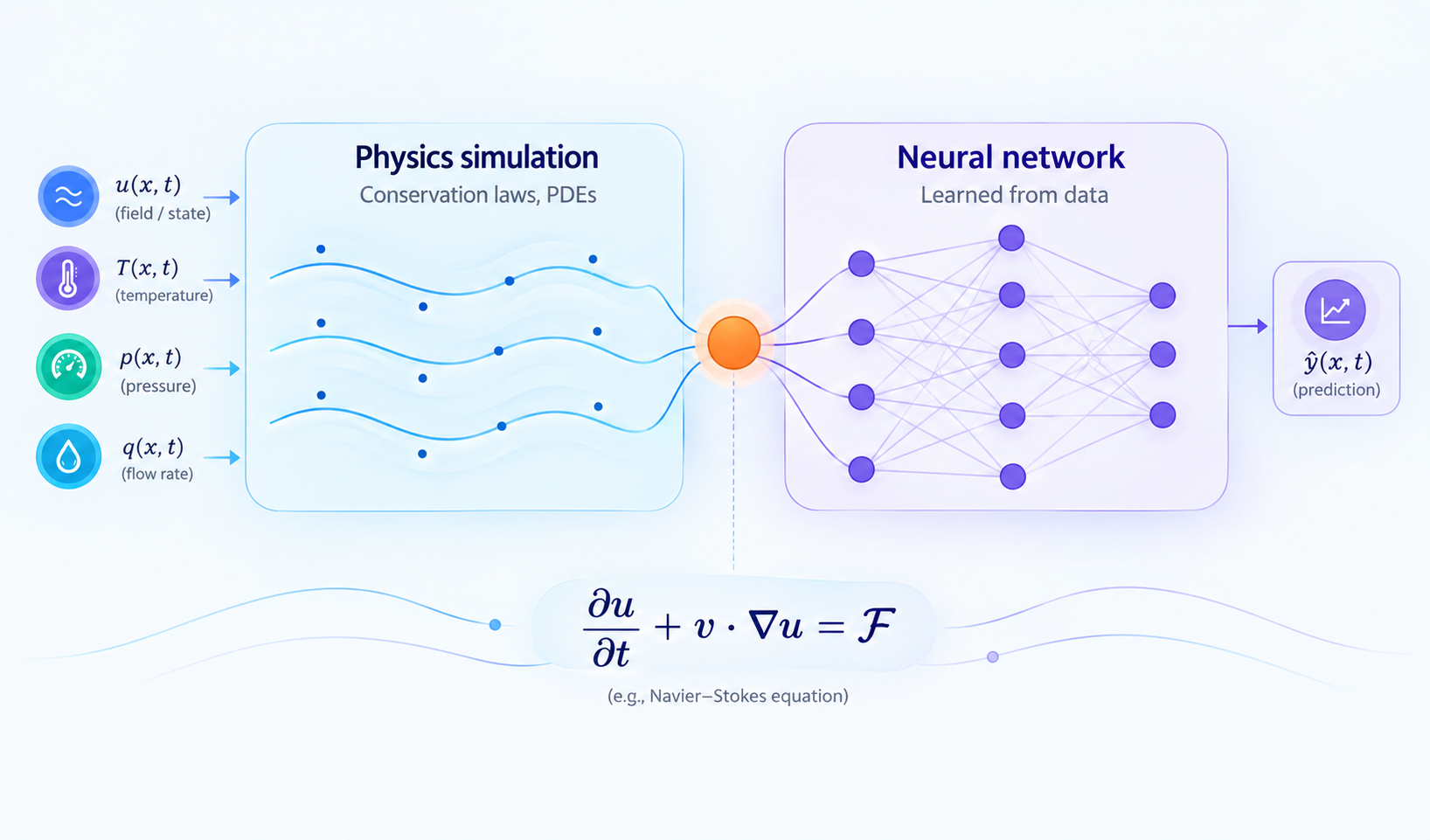
Physics-informed machine learning (PIML) is the attempt to merge these cultures: build models that learn from data the way neural networks do, while respecting the equations — conservation of mass, momentum, energy, Maxwell’s equations, structural mechanics — that engineers already know are true.

The appeal for industry is straightforward. Purely data-driven models are data-hungry, can violate basic physical constraints (negative concentrations, non-conservative energy, discontinuous stress fields), and often fail to extrapolate outside the conditions they were trained on — which is exactly where engineers need trustworthy predictions most: rare events, new operating regimes, novel designs. Purely physics-based solvers, meanwhile, are accurate but slow, sometimes requiring hours on a supercomputer for a single high-fidelity simulation, which makes them impractical for real-time control, design-space exploration, or digital twins that must update continuously.

PIML aims to sit in between: physical law as an inductive bias that lets models learn from less data, generalize further, and run orders of magnitude faster than the solvers used to generate their training data in the first place.

What follows is a tour of the main technical approaches, what has changed recently, and where the technology is actually earning its keep on factory floors, in weather centers, and in engineering design offices today.

1. The core methods and algorithms

1.1 Physics-informed neural networks (PINNs): physics as a loss term

The method most people mean when they say “PIML” is the physics-informed neural network, introduced by Maziar Raissi, Paris Perdikaris, and George Karniadakis in 2019. The idea is elegant: train a neural network to approximate the solution of a partial differential equation (PDE) by minimizing a composite loss function with three parts — a data-fitting term (if any measurements exist), a boundary/initial-condition term, and a physics residual term computed by plugging the network’s own output into the governing PDE using automatic differentiation. If the network’s predicted temperature, velocity, or stress field doesn’t satisfy the heat equation or Navier–Stokes equations at randomly sampled “collocation” points, that residual is penalized. Because automatic differentiation gives exact derivatives of the network output with respect to its inputs, no mesh or discretization is required — the physics is enforced everywhere in the domain, not just at grid points.

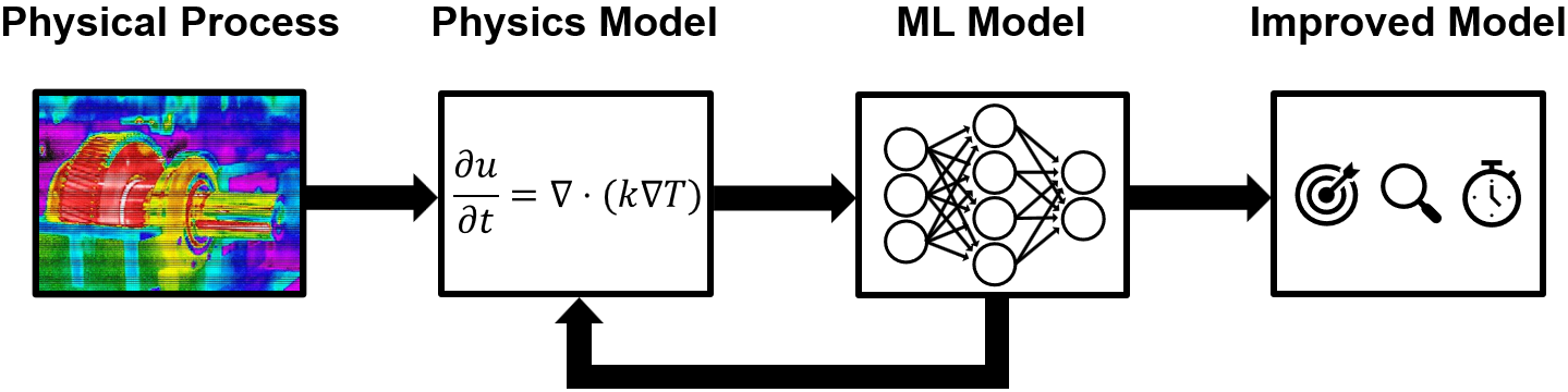
blogs.mathworks.com, What Is Physics-Informed Machine Learning?, Sivylla Paraskevopoulou

This turns PDE-solving into an optimization problem rather than a linear-algebra problem, which has two practical consequences: PINNs can solve inverse problems (inferring unknown material properties, boundary conditions, or source terms from sparse sensor data) about as naturally as forward problems, and they can incorporate noisy, irregular, real-world measurements directly into the loss function alongside the physics.

The basic PINN recipe has since been extended in several directions that address its early weaknesses (slow convergence, difficulty with stiff or multi-scale problems, spectral bias toward low-frequency solutions):

– Domain decomposition (conservative PINNs / cPINN, extended PINNs / XPINN) splits the domain into subregions, each with its own smaller network, stitched together with interface conditions — improving scalability to complex geometries.

– Adaptive and causal training reweights collocation points or loss terms during training so the network learns solutions in the correct temporal or spatial order, rather than trying to satisfy the whole domain at once.

– PIKANs (physics-informed Kolmogorov–Arnold Networks) replace the standard multilayer perceptron backbone with Kolmogorov–Arnold Networks, which use learnable activation functions on edges rather than fixed activations on nodes; recent surveys report improved accuracy and interpretability on stiff and multi-scale PDEs compared with vanilla PINNs.

– Variable-transformation and Fourier-feature embeddings help PINNs represent high-frequency or thin-boundary-layer solutions, a known weak spot of standard architectures.

– Bayesian PINNs place a distribution over network weights (or use ensembles) so predictions come with calibrated uncertainty — important for any safety-relevant industrial deployment.

PINNs are now widely used for combustion, structural mechanics, biomedical flows, and industrial gas turbine modeling, and are one of several architectures directly supported inside NVIDIA’s open-source PhysicsNeMo framework (formerly Modulus).

1.2 Hard-constrained and structure-preserving architectures

Rather than penalizing physics violations in a loss function, a second family of methods bakes the physics directly into the network’s architecture, so the constraint is satisfied *by construction* and cannot be violated no matter what the weights are. Examples include divergence-free velocity-field parameterizations for incompressible flow, Hamiltonian and Lagrangian neural networks that guarantee energy conservation, and equivariant graph neural networks that respect rotational and translational symmetry.

This idea has matured quickly for multi-body and mechanical systems: recent graph-network architectures such as Dynami-CAL GraphNet and **Equi-Euler GraphNet** are explicitly built to conserve linear and angular momentum while predicting forces and trajectories in dynamical systems — useful for robotics, vehicle dynamics, and rotating machinery, where a model that silently “creates” momentum is worse than useless. Hard constraints tend to generalize better than soft (loss-based) constraints, precisely because there is no way for the optimizer to trade off physics accuracy against data fit.

1.3 Neural operators: learning the solution operator, not one solution

A PINN, once trained, has learned the solution to one specific PDE instance — one geometry, one set of boundary conditions, one set of material parameters. Change any of those and you must retrain. Neural operators solve a more ambitious problem: they learn the mapping itself — from an arbitrary input function (an initial condition, a permeability field, a boundary shape) to the corresponding solution function — so that, once trained, the model can be evaluated instantly on new inputs it has never seen, without retraining. This is the difference between learning one function and learning a family of functions parameterized by physics.

The two dominant architectures are:

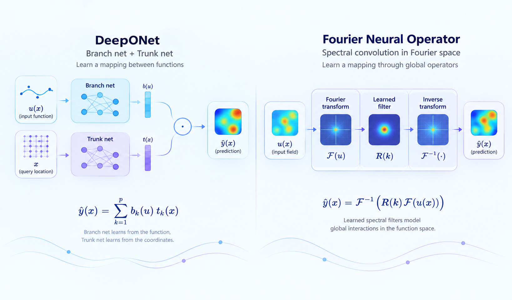
– DeepONet (Lu, Jin, Karniadakis, based on the universal approximation theorem for operators), which splits the network into a “branch” net that encodes the input function and a “trunk” net that encodes the query location, combining them to predict the output field at any point.

– Fourier Neural Operator (FNO) (Li, Kovachki, Anandkumar et al.), which performs convolutions in Fourier space, giving it a strong inductive bias for problems with smooth, translation-invariant dynamics and letting it be evaluated at any spatial resolution.

Both have spawned a large family of variants — U-FNO for multiphase subsurface flow, Fourier-DeepONet and Fourier-MIONet for seismic full-waveform inversion and geological carbon sequestration, geometry-informed neural operators (GINO) for irregular meshes, and physics-informed neural operators that add PDE-residual losses on top of operator learning to reduce the amount of training data needed. Because a trained operator generalizes across an entire family of scenarios, neural operators have become the backbone of choice for digital twins, design-space exploration, and real-time surrogate modeling, where the same model must respond to constantly changing inputs.

1.4 Graph neural networks for mesh- and particle-based simulation

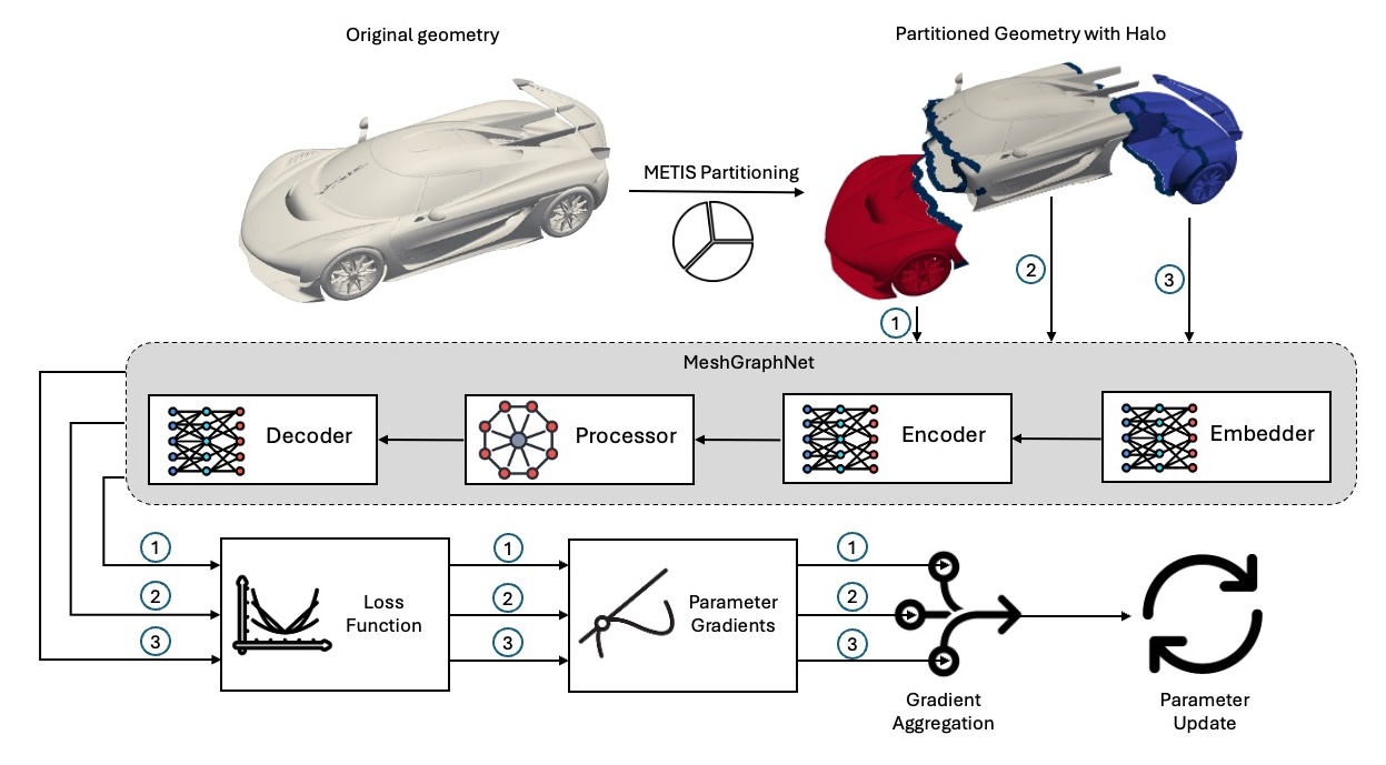
NVIDIA PhysicsNeMo documentation

Many industrial simulations — computational fluid dynamics, structural finite-element analysis, granular and particle systems — are naturally represented as meshes or point clouds rather than regular grids. Graph neural networks (GNNs) generalize convolution to this setting: each mesh node or particle is a graph node, physical interactions (stress transfer, fluid advection, contact) are encoded as message-passing along edges, and the network learns to predict how the system evolves one time step at a time. Architectures such as MeshGraphNets popularized this “learned simulator” approach, and it has since been extended with physics-informed losses (for fluid flow and heat convection), heterogeneous graphs for multi-component manufacturing systems, and phase-field-aware graph networks that accelerate microstructure evolution simulations in additive manufacturing. GNN-based simulators are particularly attractive in industry because they operate on the same unstructured meshes engineers already use in CAD and finite-element tools, lowering the barrier to adoption.

1.5 Hybrid, gray-box, and residual-learning models

Many industrial teams don’t try to replace a physics-based model outright — they use ML to correct it instead. In residual or gray-box modeling, a first-principles model (often a simplified or lower-fidelity one) makes a baseline prediction, and a neural network is trained only to learn the discrepancy between that baseline and reality. This is attractive precisely because it doesn’t ask the ML model to relearn physics that is already well understood — it only has to learn what the physics model gets wrong, which is usually a much smaller and smoother function, learnable from far less data. This pattern shows up repeatedly in process industries: physics-informed recurrent networks for dynamic chemical process systems, hybrid models for predictive control under noisy data, and physics-informed corrections for plant-model mismatch in industrial reactors.

1.6 Differentiable physics and differentiable simulation

A related but distinct idea is to make the physics simulator itself differentiable — implementing PDE solvers, rigid-body dynamics, or contact mechanics in a framework like PyTorch or JAX so that gradients can flow end-to-end from a design objective, through the simulation, back to design parameters or control policies. This enables gradient-based design optimization (e.g., optimizing an airfoil shape or a robot’s morphology by differentiating through a full CFD or dynamics rollout) and can be combined with neural components inserted directly into the simulation loop — differentiable physics and neural operators are increasingly treated as complementary rather than competing.

1.7 Physics-informed and model-based reinforcement learning

Everything so far in this section learns to predict or simulate. Reinforcement learning (RL) learns to act — training a policy that outputs control decisions (valve positions, actuator torques, setpoints) through trial and error against a reward signal, rather than fitting a solution to a known equation. The physics-informed connection enters through the environment the policy trains against. Training directly on real hardware is slow, expensive, and often unsafe, so almost all industrial RL work trains inside a simulator first, and the fidelity of that simulator largely determines whether the resulting policy survives contact with the real system — the classic sim-to-real gap.

Two variants of this pattern recur across the literature:

– Physics-simulator-in-the-loop RL, where the policy trains inside a full CFD, rigid-body, or finite-element simulator, sometimes through a differentiable-physics engine (Section 1.6) so gradients from the reward can flow back through the dynamics directly rather than relying solely on noisier policy-gradient estimates. This tends to improve sample efficiency substantially for continuous-control problems like flow control or legged locomotion.

– Model-based RL with a learned world model, where the policy trains against a neural operator or GNN-based surrogate (Sections 1.3–1.4) standing in for the real environment. Because these surrogates run orders of magnitude faster than the solvers that trained them, a policy can accumulate years of simulated experience in hours — at the cost of inheriting whatever the surrogate gets wrong.

A related, smaller idea is physics-informed reward shaping: penalizing actions that would violate known constraints (pressure limits, energy balance, actuator limits) directly in the reward function, so the policy is steered away from physically implausible behavior before it ever tries it on real hardware.

The clearest deployed example is plasma control. DeepMind’s collaboration with the Swiss Plasma Center trained an RL policy against a simulator of the TCV tokamak and then used it to directly control the tokamak’s magnetic coils and shape plasma configurations on real hardware — one of the few cases where a policy trained substantially in simulation was handed direct control authority over an expensive, safety-critical physical system, rather than staying in an advisory role. Related work applies the same pattern to HVAC and building-energy control, chemical process setpoint optimization, and power-grid balancing, though most of these deployments remain pilot-scale rather than the multi-year, unattended production runs described for other methods in Section 2.

1.8 Reduced-order modeling and latent dynamics

Classical reduced-order modeling techniques (proper orthogonal decomposition, dynamic mode decomposition) compress high-dimensional simulation states into a small number of dominant modes. Modern PIML combines this with autoencoders and neural ODEs: an encoder compresses the full physical state into a low-dimensional latent space, a (physics-constrained) neural network evolves the dynamics in that latent space, and a decoder reconstructs the full field. This is especially valuable for real-time control and monitoring applications where the full-order model is too expensive to run online but the underlying dynamics live on a much lower-dimensional manifold.

1.9 Equation discovery: learning the physics itself

A different branch of PIML doesn’t assume the governing equations are known — it tries to discover them from data. Sparse Identification of Nonlinear Dynamics (SINDy), developed by Steven Brunton, Nathan Kutz and colleagues, fits a sparse linear combination of candidate nonlinear terms (drawn from a library of polynomials, trigonometric functions, etc.) to time-series data, using sparsity-promoting regression so that only a handful of terms survive — yielding an interpretable, human-readable differential equation rather than a black-box network. Symbolic regression methods pursue the same goal with genetic programming or transformer-based approaches. These methods matter for industrial applications where no first-principles model exists yet, or where the goal is not just prediction but scientific understanding — recent perspectives in the physics literature explicitly frame the open question of whether such tools make genuinely new discoveries or simply reformulate existing knowledge, a live debate as this class of method scales up.

1.10 Physics-informed Gaussian processes and uncertainty quantification

Gaussian processes (GPs) remain popular in regimes with very little data, because physical constraints (linear PDEs, monotonicity, boundary conditions) can often be encoded directly into the GP’s covariance kernel, and GPs naturally output calibrated uncertainty. For industrial risk-sensitive settings — asset health monitoring, safety cases, anomaly detection — uncertainty quantification (UQ) is not optional, and this has become a research focus across the whole PIML landscape: Bayesian PINNs, ensemble and dropout-based UQ for neural operators, and conformalized DeepONets, which wrap operator predictions with distribution-free statistical guarantees on prediction intervals, so that downstream engineering decisions can be made with known confidence rather than a single point estimate.

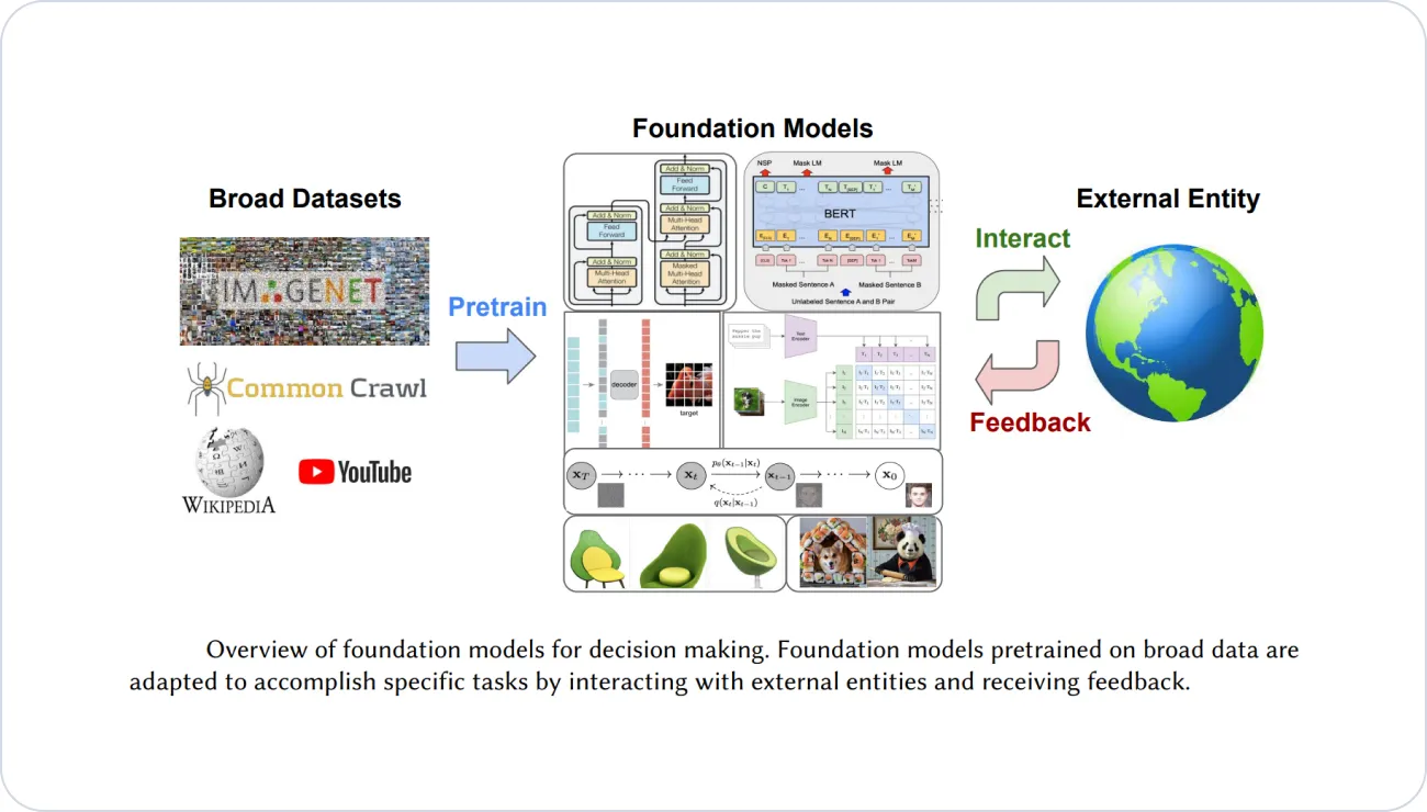
1.11 Foundation models for physics

v7labs, Foundation Models: The Benefits, Risks, and Applications

The newest and arguably most consequential development is the emergence of large pretrained foundation models for physical systems, following the same playbook that transformed language and vision: train one very large model on a huge, diverse corpus of physical simulation and observational data, then fine-tune or zero-shot it across many downstream tasks. The clearest example is weather. Google DeepMind’s GraphCast — a graph neural network trained on four decades of ECMWF ERA5 reanalysis data — matched or beat the accuracy of ECMWF’s operational Integrated Forecasting System on most variables while generating a 10-day global forecast in under a minute on a single machine, compared with roughly an hour on a large supercomputer for the classical model. Microsoft Research’s Aurora pushed the “foundation model” framing further: a 1.3-billion-parameter model pretrained on more than a million hours of heterogeneous Earth-system data (reanalysis, forecasts, wave and air-quality data), which can be fine-tuned to multiple downstream tasks — medium-range forecasting, air-pollution forecasting, ocean waves, and, notably, tropical cyclone tracking, where it has been reported to outperform every operational forecast center including the U.S. National Hurricane Center at short lead times. Huawei’s Pangu-Weather, NVIDIA’s FourCastNet (built on Adaptive Fourier Neural Operators), and ECMWF’s own in-house AIFS round out a now-crowded field of AI weather models running alongside, and in some operational contexts replacing, classical numerical weather prediction. Unlike a PINN, these models mostly do not encode explicit PDE constraints — they lean on scale and diverse pretraining rather than hand-coded physics — but they still sit within the broader PIML story because they are increasingly hybridized with physical constraints, used as fast physics surrogates, and benchmarked directly against equation-based models.

2. Real-world industrial use cases

raksha-anirveda.com, 8,000 Holes, Zero Delay: Robots Take Over Tejas Wings, RA Editorial Desk

Weather, climate, and disaster preparedness

AI weather models have moved from research curiosity to production infrastructure in a few years. NVIDIA’s Earth-2 platform packages GraphCast, FourCastNet, and other data-driven models for operational use, and national meteorological services and disaster-response organizations are exploring these tools specifically to close early-warning gaps in regions where supercomputing infrastructure for classical numerical weather prediction is unavailable — trading a few percentage points of accuracy in some regimes for forecasts that run on a single GPU in seconds instead of a supercomputer cluster in hours.

Aerospace design and computational fluid dynamics

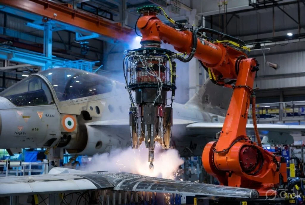
Aircraft manufacturers and their simulation-software partners are using neural-operator-based surrogates to compress design-exploration cycles that used to take days of CFD into interactive, near-real-time loops. Simulation vendor Luminary Cloud’s SHIFT-Wing model, for instance, was trained on NVIDIA’s PhysicsNeMo framework in partnership with aircraft manufacturer Otto Aviation, and delivers transonic wing-aerodynamics predictions in seconds instead of the hours a full CFD run would take. More broadly, major engineering-simulation vendors — Ansys, Altair, Cadence, Siemens, and Synopsys among them — have been integrating GPU-accelerated physics-ML into their computational-engineering product lines rather than treating it as an academic side project.

Semiconductor design and fabrication

Chipmaking is one of the most physics-intensive industrial processes in existence — TCAD (technology computer-aided design) simulations model electromagnetics, thermal transport, and device physics down to the nanometer. Semiconductor EDA vendors such as Silvaco have begun combining decades of physics-based TCAD modeling with GPU-accelerated physics-ML frameworks to build high-fidelity digital twins for chip design and fab-line optimization, while, on the factory floor, major electronics manufacturers have been using physics-informed digital twins (combining simulation platforms with GNN- and operator-based physics-ML models) to optimize factory layout, robotics deployment, and operational efficiency at scale.

Materials discovery and energy storage

Materials science has arguably produced PIML’s single largest quantitative result to date: Google DeepMind’s GNoME (Graph Networks for Materials Exploration) used graph neural networks trained with an active-learning loop against physics-based stability calculations to predict roughly 2.2 million candidate inorganic crystal structures, of which several hundred thousand were assessed as stable enough to be promising synthesis targets — including hundreds of new lithium-ion conductor candidates relevant to next-generation battery design, and new layered compounds relevant to superconductors and electronics. This expanded the number of known stable materials by close to an order of magnitude in a single release, and independent labs have already synthesized hundreds of the predicted structures. The result illustrates both the promise and the current limits of PIML in materials industry adoption: proprietary formulation data and the mismatch between idealized lab conditions and messy production environments remain real barriers to converting these predictions into deployed products.

Energy, subsurface, and geoscience

Neural operators have found a natural home wherever classical solvers are prohibitively expensive to run many times over, which describes most subsurface engineering. Fourier-enhanced DeepONets and U-FNOs are now used as fast surrogates for full-waveform seismic inversion, multiphase flow in porous media, and geological carbon-sequestration modeling, where the same PDE must be resolved repeatedly across thousands of geological scenarios for uncertainty quantification — a task that would be computationally infeasible with a traditional solver run one scenario at a time. Fourier neural operators have also been applied as fast surrogates for tokamak plasma dynamics in nuclear-fusion research, replacing expensive physics codes for scenario screening — and, taken a step further into control rather than prediction, this is the same simulation groundwork that let DeepMind’s reinforcement-learning policy (Section 1.7) take direct control of a real tokamak’s magnetic coils.

Structural, civil, and mechanical engineering

Digital twins of physical infrastructure — from reinforced-concrete containment vessels under seismic loading to rotating machinery and gas turbines — increasingly combine finite-element model updating with neural-operator surrogates, letting engineers run “what-if” seismic or fatigue scenarios interactively rather than waiting on a full finite-element solve. Physics-informed neural networks have also been applied directly to beam and structural-mechanics problems in both forward design and inverse damage-identification settings.

Manufacturing and additive manufacturing

Physics-informed losses and physics-embedded graph networks are used across additive manufacturing (3D printing) to predict and control thermal distortion, residual stress, and microstructure evolution during the print process — spanning product design, process planning, and in-line quality control. NVIDIA PhysicsNeMo-based digital twins are explicitly marketed for predicting thermal distortion in additive manufacturing and optimizing process parameters in real time, and broader smart-manufacturing roadmaps highlight physics-informed graph networks for anomaly detection and virtual sensing on production lines where dense instrumentation is too costly.

Process industries and chemical engineering

Chemical and process engineers have adopted physics-informed recurrent networks and hybrid gray-box models for dynamic process control, batch crystallization under uncertainty, stiff chemical-kinetics surrogates, and — in one concretely validated example — a physics-informed and data-driven model of an actual industrial wastewater treatment plant, validated against real plant data rather than simulation alone.

Electrical systems and power grids

A 2026 review of PIML for electrical machines and drives highlights its use for high-fidelity modeling, monitoring, and control across Industry 4.0 settings, citing gains in data efficiency, interpretability, and physical consistency, alongside continuing challenges around parameter sensitivity and robustness to changing operating conditions. Related work applies physics-informed losses to non-intrusive load monitoring — disaggregating whole-building power measurements into individual appliance loads without needing physically implausible predictions — while early-stage reinforcement-learning pilots (Section 1.7) are being tested for real-time grid-balancing and demand-response control.

Automotive, robotics, and multi-body dynamics

Vehicle-dynamics modeling, predictive maintenance, and system identification in the automotive sector rely heavily on physics-informed neural networks and operator-learning methods, while structure-preserving graph networks that explicitly conserve momentum (rather than merely approximating it) are being developed specifically for multi-body force and trajectory prediction — directly relevant to robotics and vehicle control, where a physically inconsistent prediction can translate into an unsafe actuator command.

Water and utilities: the deployment reality check

Perhaps the most instructive recent account of what it actually takes to get PIML into production comes from utility operators, not tech companies. Researchers piloting physics-informed models at a wastewater treatment plant (Veas, near Oslo) reported that getting a model to fit historical data was the easy part; the harder, ongoing problem is deciding when and why a deployed model’s performance has drifted — distinguishing sensor drift or calibration issues from genuine changes in operating conditions or underlying physics. Their conclusion, echoed across the field, is that the physical model is not just a training-time convenience but the interpretive framework that lets engineers diagnose why a live model’s predictions are going wrong — something a black-box data-driven model cannot offer on its own. In some deployments, teams have gone further still, using an existing physics-based simulator as the literal backbone of the deployed model rather than trying to replace it outright with a neural network.

3. What’s genuinely new versus what’s still promise

It’s worth being honest about where PIML has crossed from research demonstration into deployed infrastructure, and where it hasn’t yet.

Where it has landed : weather forecasting is the clearest case of full production deployment, with AI models now running alongside — and in some products, ahead of — classical numerical weather prediction at operational meteorological centers. Materials-discovery pipelines have produced concrete, verifiable, independently-replicated scientific results. GPU-vendor-backed frameworks (PhysicsNeMo) are now bundled into mainstream commercial engineering-simulation software from multiple major vendors, not just used in isolated pilot projects. Neural-operator surrogates for subsurface and seismic modeling are handling production-scale 3D problems, not toy benchmarks.

Where it’s still maturing : general-purpose “one model for every PDE” foundation models outside weather remain an active research direction rather than an industrial standard. Hard theoretical guarantees on when and how much a neural operator will fail to extrapolate outside its training distribution are still incomplete. And, as the wastewater and gas-turbine case studies both suggest, the gap between a published method that fits benchmark data well and a system that a plant operator will trust to run unattended for years is still substantial — validation, monitoring for model drift, and clear protocols for when to fall back to a physics-only model are, at present, mostly built by hand for each deployment rather than solved once and reused.

A methodological convergence worth watching: rather than neural networks replacing solvers outright, some of the most promising recent work fuses them directly — for example, the neural-operator element method, which embeds operator-learning components inside a classical finite-element framework so that the accuracy guarantees of the numerical method and the speed of the learned surrogate are both available where needed, rather than forcing engineers to choose one or the other.

4. The road ahead

The trajectory across nearly every method described above points in the same direction: from single-instance solvers (PINNs solving one PDE at a time) toward operators and foundation models that generalize across whole families of physical scenarios; from soft physics constraints in a loss function toward hard, architecturally guaranteed conservation laws; and from research prototypes toward vendor-supported, GPU-accelerated software stacks (PhysicsNeMo, Omniverse, and equivalents from major simulation vendors) that industrial engineering teams can actually deploy without building everything from scratch. Uncertainty quantification, once an academic afterthought, is becoming a first-class requirement as these models move from advisory tools into systems that influence real engineering and operational decisions.

None of this replaces domain expertise or first-principles physics — if anything, the clearest lesson from early industrial deployments is that the physics is what makes the machine learning trustworthy, interpretable, and diagnosable when things go wrong, not an optional add-on to be discarded once a model performs well on a benchmark. The honest way to describe the horizon, then, is not “physics-informed ML will replace simulation” but “the boundary between simulation and machine learning is dissolving,” with the winning systems in each industry being the ones that use the right blend of the two for the problem, the data, and the risk at hand.

Physics-Informed Machine Learning and Its Horizon in Industrial Applications